Chapter 08 基础算法

介绍SARSA、Q-Learning算法原理和实现。

禁止转载，侵权必究！Update 2020.11.21

前言

强化学习作为一个独立的机器学习的分支和我们前面课程介绍的CNN有什么不同呢？

CNN的一般性流程：输入图片–>神经网络–>预测（分类、目标检测）

强化学习一般性流程：初始化游戏–>state1–>action1—>state2(reward1)–>action2–>state3(reward2)–>action3…–>结束

教学环境

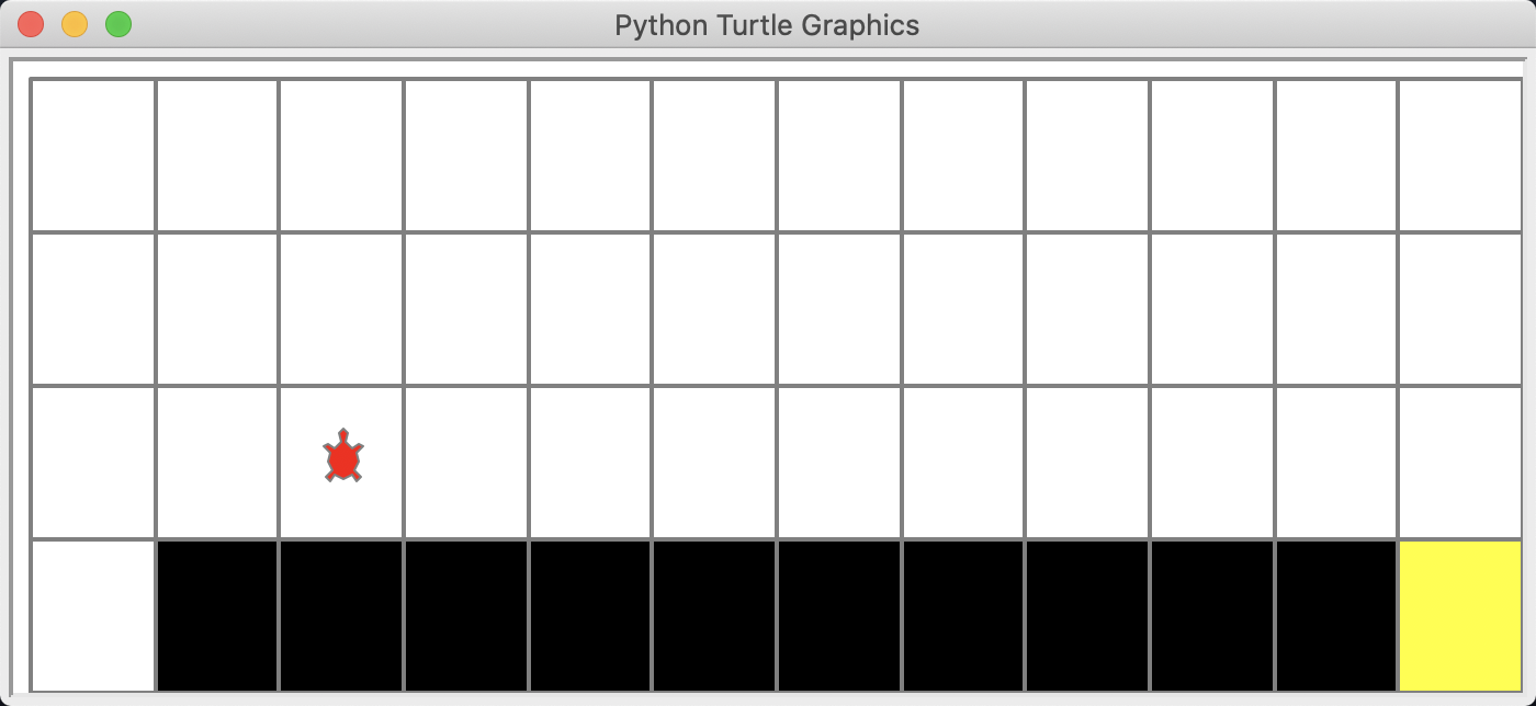
gym是一个开放的强化学习教学环境，比如我们后面要用到的小乌龟找出口和CartPole都可以用gym库来模拟。另外，在真实的强化学习任务中建立仿真环境也非常重要。

SARSA算法

1.Agent

import numpy as np

class SarsaAgent(object):
    def __init__(self, obs_n, act_n, learning_rate=0.01, gamma=0.9, e_greed=0.1):
        self.act_n = act_n      # 动作维度，有几个动作可选
        self.lr = learning_rate # 学习率
        self.gamma = gamma      # reward的衰减率
        self.epsilon = e_greed  # 按一定概率随机选动作
        self.Q = np.zeros((obs_n, act_n))

    # 根据输入观察值，采样输出的动作值，带探索
    def sample(self, obs):
        ...

    # 根据输入观察值，预测输出的动作值
    def predict(self, obs):
        Q_list = self.Q[obs, :]
        maxQ = np.max(Q_list)
        action_list = np.where(Q_list == maxQ)[0]  # maxQ可能对应多个action
        action = np.random.choice(action_list)
        return action

    # 学习方法，也就是更新Q-table的方法
    def learn(self, obs, action, reward, next_obs, next_action, done):
        ...

    # 保存Q表格数据到文件
    def save(self):
        npy_file = './q_table.npy'
        np.save(npy_file, self.Q)
        print(npy_file + ' saved.')
    
    # 从文件中读取Q值到Q表格中
    def restore(self, npy_file='./q_table.npy'):
        self.Q = np.load(npy_file)
        print(npy_file + ' loaded.')

learn方法:

    # 学习方法，也就是更新Q-table的方法
    # obs就是state的意思
    def learn(self, obs, action, reward, next_obs, next_action, done):
        """ on-policy
            obs: 交互前的obs, s_t
            action: 本次交互选择的action, a_t
            reward: 本次动作获得的奖励r
            next_obs: 本次交互后的obs, s_t+1
            next_action: 根据当前Q表格, 针对next_obs会选择的动作, a_t+1
            done: episode是否结束
        """
        predict_Q = self.Q[obs, action]
        if done:
            target_Q = reward # 没有下一个状态了
        else:
            target_Q = reward + self.gamma * self.Q[next_obs, next_action] # Sarsa
        self.Q[obs, action] += self.lr * (target_Q - predict_Q) # 修正q

sample方法：

    # 根据输入观察值，采样输出的动作值，带探索
    def sample(self, obs):
        if np.random.uniform(0, 1) < (1.0 - self.epsilon): #根据table的Q值选动作
            action = self.predict(obs)
        else:
            action = np.random.choice(self.act_n) #有一定概率随机探索选取一个动作
        return action

2.训练

导入依赖包

import gym
import numpy as np
import time
from sarsa_agent import SarsaAgent
from gridworld import CliffWalkingWapper

定义训练方法

def run_episode(env, agent, render=False):
    total_steps = 0 # 记录每个episode走了多少step
    total_reward = 0

    obs = env.reset() # 重置环境, 重新开一局（即开始新的一个episode）
    action = agent.sample(obs) # 根据算法选择一个动作

    while True:
        next_obs, reward, done, _ = env.step(action) # 与环境进行一个交互
        next_action = agent.sample(next_obs) # 根据算法选择一个动作
        # 训练 Sarsa 算法
        agent.learn(obs, action, reward, next_obs, next_action, done)

        action = next_action
        obs = next_obs  # 存储上一个观察值
        total_reward += reward
        total_steps += 1 # 计算step数
        if render:
            env.render() #渲染新的一帧图形
        if done:
            break
    return total_reward, total_steps

执行训练

# 使用gym创建悬崖环境
env = gym.make("CliffWalking-v0")  # 0 up, 1 right, 2 down, 3 left
env = CliffWalkingWapper(env)

# 创建一个agent实例，输入超参数
agent = SarsaAgent(
        obs_n=env.observation_space.n,
        act_n=env.action_space.n,
        learning_rate=0.1,
        gamma=0.9,
        e_greed=0.1)

is_render = False
# 训练500个episode，打印每个episode的分数
for episode in range(500):
    ep_reward, ep_steps = run_episode(env, agent, is_render)
    print('Episode %s: steps = %s , reward = %.1f' % (episode, ep_steps, ep_reward))

    if episode % 20 ==0:
        is_render = True
    else:
        is_render = False

3.测试

定义测试方法

def test_episode(env, agent):
    total_reward = 0
    obs = env.reset()
    while True:
        action = agent.predict(obs) # greedy
        next_obs, reward, done, _ = env.step(action)
        total_reward += reward
        obs = next_obs
        time.sleep(0.5)
        env.render()
        if done:
            break
    return total_reward

执行测试

# 全部训练结束，查看算法效果
test_reward = test_episode(env, agent)
print('test reward = %.1f' % (test_reward))

4.查看结果：

Q-Learning算法

1.Agent差别

def learn(self, obs, action, reward, next_obs, next_action, done): # sarsa
def learn(self, obs, action, reward, next_obs, done): # Q-Learning

learn方法差别

target_Q = reward + self.gamma * self.Q[next_obs, next_action] # Sarsa
target_Q = reward + self.gamma * np.max(self.Q[next_obs, :]) # Q-learning 

2.训练方法差别

sarsa:

    ...
    action = agent.sample(obs) # 根据算法选择一个动作

    while True:
        next_obs, reward, done, _ = env.step(action) # 与环境进行一个交互
        next_action = agent.sample(next_obs) # 根据算法选择一个动作
        # 训练 Sarsa 算法
        agent.learn(obs, action, reward, next_obs, next_action, done)

        action = next_action
        ...

注意： 它的next_action需要额外用sample()方法初始化。

Q-Learning:

    ...
    while True:
        action = agent.sample(obs) # 根据算法选择一个动作
        next_obs, reward, done, _ = env.step(action) # 与环境进行一个交互
        # 训练 Q-learning算法
        agent.learn(obs, action, reward, next_obs, done)
        ...

4.查看结果：

SARSA和Q-Learning算法比较

• 所有强化学习算法都存在探索与利用的平衡问题，一般采用两个策略模型，一个策略为行为策略，用于保持探索性，提供多样化的数据，优化另一个策略(目标策略)。
• Sarsa是先用sample()函数做出动作后再更新Q，循环往复，依据Q表格的值走，直到走到失败、成功或者到达最大step数。Q-Learning先假设下一步选取Max Reward的动作的Q值去更新Q。然后再用sample()函数选择动作。循环往复，直到走到失败、成功或者到达最大step数。
• sample()函数实现了ε-greedy算法。有一些概率的走法是探索，有一些概率的走法是利用。在利用这种走法下还是走Max Q，也就是顺着之前的经验走(predict()函数)。
• SARSA算法是on-policy的，也就是说他的行为策略和目标策略是一致的，都是sample()。Q-Learning算法是off-policy的，目标策略选Q表格里面的最大值，所以它的目标策略Max Q，行为策略跟SARSA一样，也是sample()函数。
• Q-Learning比SARSA激进，更愿意选择最优解。
• SARSA比Q-Learning收敛更快，训练轮数更少。
• 在程序最后，我们用test_episode()来验证效果。它内部是在调用predict()。是不是巧合呢？不，这不是巧合。因为测试的走法就应该是按经验Q值来走！符合正常的思维逻辑！